
Why production drift detection matters
The practical problem is simple: a model that performed well at release can become less reliable after deployment, even if the code never changes. New customer behavior, seasonality, upstream schema shifts, instrumentation changes, and adversarial or just messy inputs can all move the operating environment away from the training distribution. In production, that creates a gap between what the model was validated against and what it now sees.
Detecting AI model drift is the process of spotting those shifts early enough to reduce business and operational risk. Done well, it helps you distinguish benign variability from a change that requires retraining, rollback, feature fixes, or human review. After reading this article, you should be able to decide whether drift detection is appropriate for your system, understand which signals are worth monitoring, apply a practical workflow, and verify whether the monitoring is trustworthy before using it as a release gate or incident trigger.
Key takeaways
AI model drift is not one thing. In production, you usually care about at least three different signals: changes in input features, changes in prediction patterns, and changes in model quality when labels are available.
A good drift detector does not try to prove the model is wrong. It tells you whether the model’s operating conditions have changed enough to justify a response.
No single metric is sufficient in isolation. Feature distribution checks, prediction stability checks, and delayed outcome metrics work best when combined with context from schema validation, upstream pipeline health, and business thresholds.
Drift detection is only operationally useful if it is calibrated. You need to know what normal variation looks like, what should page a human, and what should be logged for later review.
What model drift actually means
In production machine learning systems, drift is a mismatch between the environment the model was trained for and the environment it currently serves. That mismatch can appear in several forms.
Input drift, sometimes called data drift, occurs when the statistical properties of incoming features change. For example, a fraud model trained on a stable mix of domestic card transactions may suddenly see a larger share of cross-border payments, new merchant categories, or different time-of-day patterns.
Prediction drift occurs when the distribution of model outputs changes significantly. A classifier that used to produce mostly low-risk scores may begin emitting more medium and high-risk scores, even before labels arrive. That shift can be caused by changing inputs, but it can also result from upstream feature engineering changes or broken feature retrieval.
Concept drift occurs when the relationship between inputs and the true target changes. This is the most operationally important version because the model can continue to look stable on the surface while becoming less accurate. A common example is Detecting Anomalies in Big Data Pipelines with Apache Spark style pipeline monitoring helping you catch upstream anomalies, but not necessarily explaining whether the business process itself has changed. In many systems, both kinds of monitoring are needed.
There is also label drift, where the target class proportions change over time. That matters because a class imbalance shift can change calibration and operating thresholds without necessarily changing feature distributions in a dramatic way.
How to detect drift in practice
The most useful approach is layered. Start with a baseline of what “normal” means, then monitor for deviations using several complementary signals. The goal is not just to observe change, but to decide whether the change is actionable.
A practical production workflow looks like this:
Baseline training data and recent stable serving data
        ↓
Validate schema, missingness, ranges, and feature freshness
        ↓
Compare current inputs to baseline distributions
        ↓
Compare prediction distributions and calibration behavior
        ↓
If labels are available, measure delayed performance
        ↓
Classify drift severity and decide: observe, investigate, retrain, rollback
The first step is to define the baseline carefully. Training data alone is not always the right reference. If your training set includes old historical behavior but the model was validated on a more recent holdout, compare production traffic to the validation window or to a known stable serving period as well. That reduces false positives caused by legitimate seasonality.
The second step is to monitor the input features that matter most to the model and the business. Not every column deserves the same scrutiny. Focus on high-impact features, features with known fragility, and features that are expensive or impossible to reconstruct after the fact. For each, track simple signals such as missing rate, unique value count, range, percentiles, categorical entropy, and distribution distance against the reference window.
The third step is to monitor outputs. Even when labels are delayed, predictions are immediate. If output scores suddenly cluster around a narrow range, or the class mix shifts sharply, that is often a useful early warning. Prediction drift does not prove degraded performance, but it often tells you where to look first.
The fourth step is to incorporate labels when they arrive. In many systems, ground truth may lag by hours or days. When it does arrive, compare delayed precision, recall, calibration, error rates, or other task-specific measures against the baseline. If you only monitor feature drift, you can miss cases where the model still sees “normal” inputs but the target relationship has changed.
What signals are worth watching
A production drift monitor should emphasize signals that are stable, interpretable, and cheap enough to run continuously.
For numeric features, a small set of descriptive statistics is often enough to identify meaningful movement: mean, standard deviation, min, max, median, and a few percentiles. Distribution distance metrics such as population stability index, KL divergence, Jensen-Shannon divergence, Wasserstein distance, or nonparametric tests can help quantify change, but each one has caveats. The best choice depends on feature type, sample size, and whether you need sensitivity to tail movement or broad shape change.
For categorical features, monitor category frequency changes, new unseen categories, and sudden growth in the “other” or null bucket. These are especially useful in systems where upstream enrichment or third-party data feeds can change without notice.
For text, embedding-based drift or token distribution drift can be useful, but these signals are heavier and usually require more careful baseline management. In high-risk systems, they are often paired with checks on prompt length, language mix, or input rejection rates.
For predictions, watch score distribution, class balance, confidence spread, and calibration drift. In security-sensitive environments, abrupt increases in uncertain predictions can be just as important as a shift toward one class. That is especially true when the model is used for triage rather than final decision-making. If your model is part of an automated review workflow, the same discipline described in Using LLM Fine-Tuning for Secure Code Review Automation applies: constrain the model, validate the output, and monitor it as an operational control rather than a static artifact.
For labels, prefer metrics that match the operational decision. A ranking model may care more about precision at a cutoff, while a risk model may care more about calibration and false negative rate. Use the metric that maps to the business consequence, not just the easiest statistic to compute.
A practical scenario you may recognize
Consider a payment-risk service deployed with a gradient-boosted model that scores transactions in real time. For several months, the model behaves consistently. Then the platform adds a new checkout flow, a mobile app release changes session timing, and the payments team onboards a new set of merchants with different geography and average basket sizes.
At first, nothing breaks visibly. Requests are still flowing. The model still returns scores. But the distribution of a few key features shifts: more missing device signals, lower transaction amounts, and a sharp increase in first-time buyers. At the same time, the output scores become more extreme, and the manual review queue grows because more transactions land near the risk threshold.
This is the kind of environment where drift detection matters operationally. If you only monitor infra health, you will miss the signal. If you only monitor accuracy after labels arrive, you may react too late. A layered drift strategy would flag the input shift, show that predictions changed with it, and then confirm whether the eventual chargeback or fraud rate also moved.
That same pattern appears in many systems: customer support automation, anomaly scoring, recommendation ranking, and security classification. The names change, but the operational question does not. Is the model still operating inside the conditions it was designed for?
Trade-offs in detection methods
No drift method is universally best. Sensitivity, interpretability, computational cost, and false positive rate are all in tension.
Simple thresholding on means, missing rates, or score distributions is easy to explain and cheap to run. It is a good fit for operational dashboards and alerting, especially when the main concern is obvious upstream breakage. The downside is that it can miss subtle but important distribution shifts.
Distance-based metrics are more expressive. They can catch shape changes that a single summary statistic would miss. The trade-off is calibration: a distance value is only meaningful relative to your baseline, sample size, and natural variation in that feature.
Hypothesis tests can add statistical rigor, but they are often misunderstood in production. With enough data, tiny harmless changes can become “significant.” With too little data, important change may not register. Statistical significance is not the same as operational significance.
Unsupervised drift detectors are useful when labels are delayed or sparse. However, they can produce alerts for changes that do not affect business outcomes. That is acceptable only if your response playbook knows how to triage those alerts efficiently.
Supervised performance monitoring is the most direct way to detect real degradation, but it depends on labels and clean joins between predictions and outcomes. In many systems, those labels arrive too late to be your first warning signal.
What this means in practice
In practice, drift detection works best as an early-warning system with human interpretation attached to it. It should answer three questions quickly: what changed, when it changed, and whether the change is likely to matter.
That means you should not try to monitor every feature equally. Start with a small set of business-critical features, the model outputs, and a few control metrics that tell you whether the pipeline is healthy. If a data source is noisy or volatile by nature, its alert threshold should be different from a stable source. If a feature is known to change seasonally, compare against the same period in prior cycles rather than a static all-time baseline.
It also means drift should be tied to a response policy. Some alerts should only create tickets. Others should trigger model shadow evaluation, manual sampling, or a canary rollback. A small number may justify retraining or feature engineering changes. Without that policy, drift detection becomes observability theater: lots of charts, little operational value.
When labels are delayed, use a two-layer strategy. First, detect input and output drift in near real time. Then, once outcomes land, compare actual performance to the earlier signals. Over time, that gives you a learned mapping between “this kind of drift” and “this kind of business impact,” which is far more useful than a raw metric threshold.
Decision guidance: when to use drift detection
Drift detection is worth implementing when the model has ongoing business impact, the data distribution is expected to evolve, or the cost of silent degradation is meaningful. That is especially true for systems with changing user behavior, external data feeds, seasonal demand, or feedback loops.
It is less useful as a standalone control when the model runs in a static environment, when the data barely changes, or when outcomes are immediate and fully observable. In those cases, standard performance checks and release validation may be enough.
A good rule is this: if you cannot explain what an alert will cause operationally, you are not ready to treat drift as a production control. Either narrow the scope, define a response, or improve the quality of the signals before promoting it to incident tooling.
Common mistakes
One common mistake is comparing live traffic directly to training data without considering release timing, seasonality, or upstream changes. That often produces noisy alerts and hides real change behind false positives.
Another mistake is treating feature drift as equivalent to model failure. A feature shift can be harmless if the model was trained with enough coverage or if the shifted feature has little predictive weight. Conversely, a small feature change can matter a lot if it affects a sensitive downstream decision.
Teams also sometimes ignore schema and freshness checks because they are not “drift” in a strict statistical sense. In practice, a missing feature or stale enrichment often causes more operational harm than subtle distribution changes.
A further mistake is using one threshold for all features. Stable, high-impact features deserve tighter controls than noisy or low-value features. Uniform thresholds create either alert fatigue or blind spots.
Finally, some teams do not define how drift alerts are validated. If every alert requires manual detective work from scratch, the monitoring system will lose credibility quickly. A small runbook with ownership, baseline references, and escalation criteria is usually enough to prevent that.
Compact production readiness checklist
Before you rely on model drift detection in production, verify the following:
- Baseline windows are documented and representative of the expected serving environment.
- The monitored features are the ones that actually matter to model behavior or business risk.
- Schema, freshness, missingness, and range checks run before deeper drift analysis.
- Feature drift, prediction drift, and delayed label performance are all monitored where feasible.
- Alert thresholds are calibrated against normal variation, not chosen arbitrarily.
- Seasonal and release-related changes are accounted for in the comparison strategy.
- Alerts map to a defined action: investigate, sample, retrain, rollback, or suppress.
- Ownership is clear for data issues, model issues, and upstream pipeline issues.
- Drift history is retained so you can compare incidents, not just single snapshots.
- A false-positive review process exists so thresholds can be improved over time.
Final takeaway
Detecting AI model drift in production is less about finding a perfect statistical test and more about building a reliable operational signal. If you combine stable baselines, focused feature checks, output monitoring, and delayed performance validation, you can catch meaningful change early enough to act on it. The practical question is not whether drift exists somewhere in the system; it is whether your current monitoring can tell you when the model has moved far enough from its expected behavior to justify a response.
Use this guidance together with JWT authentication in ASP.NET Core APIs and async try-catch to connect the workflow with related operational context already available on the site.
Part of the Programming: AI / Machine Learning Insights content cluster.